Digital Signal Processing

Last updated on Nov 5, 2021 19 min read R

Photo by Gritte on Unsplash

Signals are everywhere around the world today. Audio communications are more critical than ever. Airplanes use signals in the air to obtain important information to ensure safety on a flight. Cell phones are pretty much a single small high performance digital signal processing device. They process our speech when we talk by removing background noise and echos that would distort the clarity. They obtain wifi signals to allow for web searches. They send SMS text messages using signals. They use digital image processing to capture excellent photos and video.

Having a basic understanding of DSP and it’s concepts can be helpful in many modern contexts.

Digital signal processing (DSP) is concerned with the representation, transformation and manipulation of signals and information they contain. DSP applications include audio and speech processing, sonar, radar and other sensor array processing, spectral density estimation, statistical signal processing, digital image processing, data compression, video coding, audio coding, image compression, signal processing for telecommunications, control systems, biomedical engineering, and seismology, among others.

When doing digital signal processing, R has not often been the first computer language that engineers work with. For decades, DSP work has been done in environments in MATLAB, Python and even C++. Even so, because of the nature of open source development and association with research, there are now several tools available today in R’s ecosystem. The bulk of R’s basic signal processing capability comes from the signal package which was ported over from the open source project Octave. Today it’s safe to say that it has never been easier to adopt R in almost any domain as demonstrated by Jared Lander’s talk at e-Rum 2020.

The functions in the R’s signal package retain the look and feel of MatLab originals. Working with these functions should make it easy for anyone familiar with MatLab to make the transition.

In addition to the basics, R contains some very nice implementations of signal processing algorithms that have applications in statistical analysis. For starters, R’s time series capabilities are second to none. Neither Matlab nor the legacy statistical software package SAS can match the scope and depth of the time series tools listed in R’s Time Series Task View.

Let’s setup several of them and walk through a demonstration.

knitr::opts_chunk$set(
  echo = TRUE,
  message = FALSE,
  warning = FALSE,
  fig.height = 7.402,
    fig.width = 12
)
suppressMessages({

library(tidyverse) 

library(here)
library(kableExtra)

library(seewave)
library(signal)
library(tuneR)
library(audio)
library(fftw)
library(cowplot)
library(EnsembleML)
})

extrafont::loadfonts(quiet = TRUE)

theme_set(hrbrthemes::theme_ft_rc() +
            theme(plot.title.position = "plot"))

pal <- wesanderson::wes_palette("Zissou1", 21, type = "continuous")

Background: Putting it in very simple terms

There are two main types of signals: continuous time signals and discrete time signals. Continuous Time Signals, as you might suspect, are continuous. They are defined at all instances of time over a given period. These types of signals are commonly referred to as analog signals. An example of an analog signal would be a simple sine curve plotted below. Notice that the sine curve is defined for every value on the interval from 0 to 2 \(\pi\). This is an analog signal.

t <- seq(0, 1, len = 100)
sig <- sin(2 * pi * t)

ggplot(mapping = aes(t, sig)) +
  geom_line(size = 3) +
  labs(title = "An Analogue, or Continuous, Signal",
       x = NULL, y = NULL)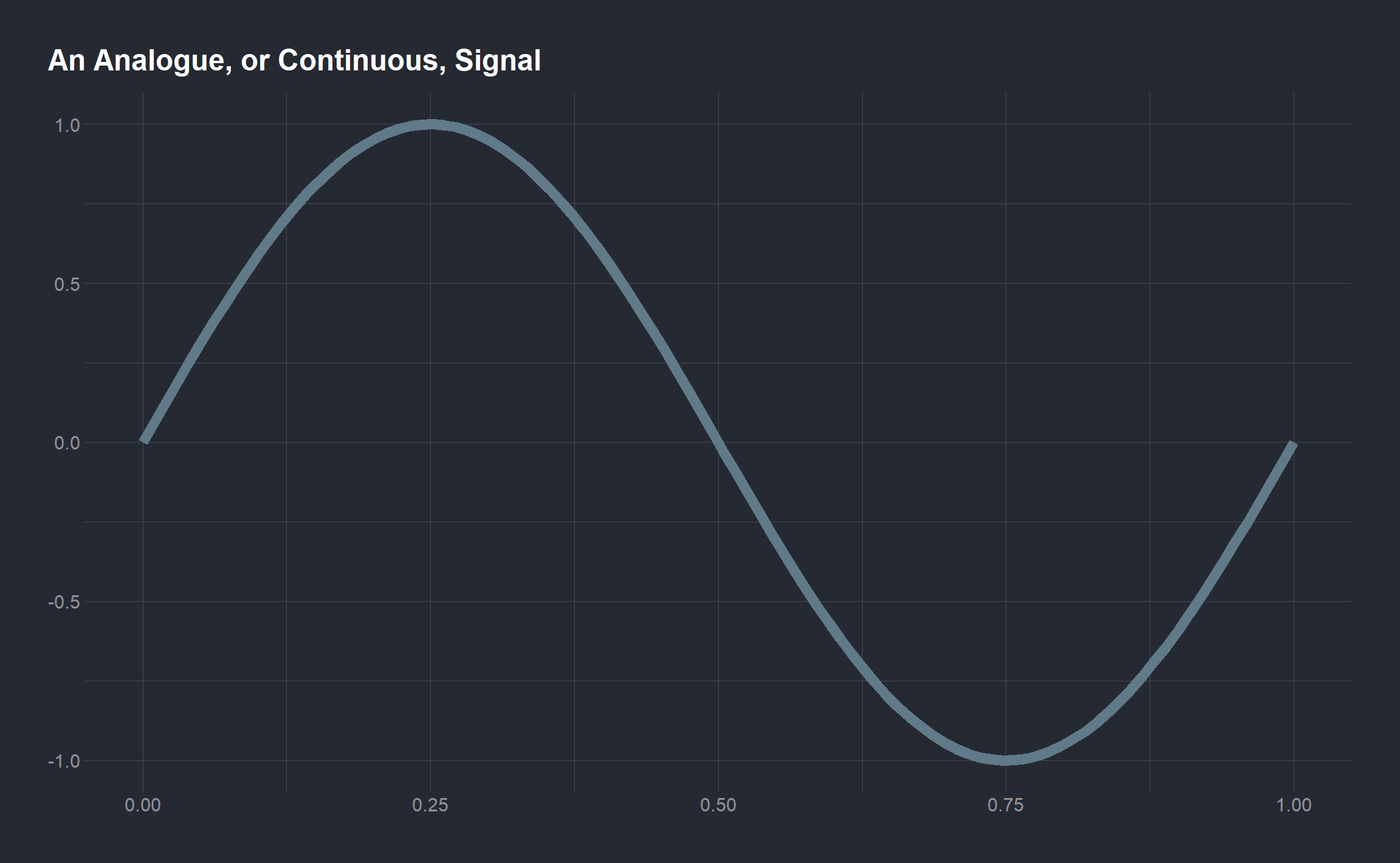

Discrete Time Signals are not continuous. They are defined only at discrete times, and thus they are represented as a sequence of numbers. This is an example of the exact same sine curve, but in a discrete form. Notice how there are only values at specific points, and anywhere besides those points the signal is not defined. In a real-world application, these points would correspond to measurements of the signal.

x <- seq(0, 1, len = 10)
y <- sin(2 * pi * x)

ggplot(mapping = aes(x, y)) +
  geom_point(size = 3) +
  labs(title = "A Discrete, or Digital, Signal",
       x = NULL, y = NULL)

Discrete-time signal processing is the rapid processing of numeric sequences indexed on integer variables. Most applications involve the use of discrete-time technology for processing signals that originate as continuous-time phenomena. In this case, a continuous-time (analogue) signal is typically converted into a sequence of samples.

Now that we have a general understanding of what a signal is and it’s properties, let’s now focus on some of the important concepts in digital signal processing, and implementing them in R. Three of the most central topics to DSP include:

Fourier Transforms: signal processing involves looking at the frequency representation of signals for both insight and computations.
Noise: defined as any signal that is not desired. A huge part of signal processing is understanding how noise is affecting the data and efficient ways of removing it.
Filters: remove specific portions of a signal at once

It is not likely that when obtaining a real-world signal you would get a perfect sinusoid without any noise. As a illustration, let’s take the sine and add some noise to it.

noisySig <- sin(2 * pi * t) + 0.25 * rnorm(length(t))

ggplot() + 
  geom_line(aes(t, noisySig), size = 2) +
  labs(title = "Noisy Signal")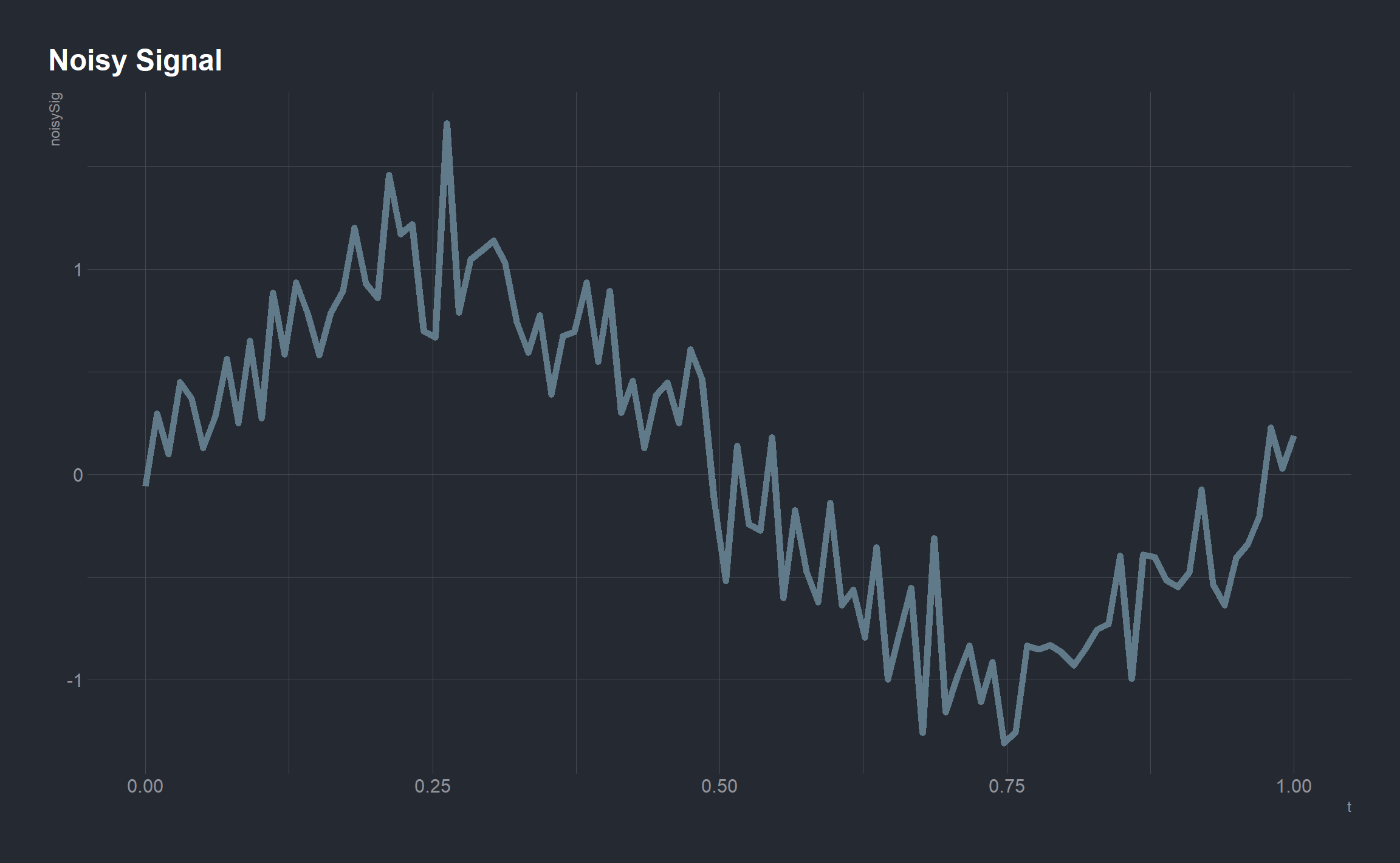

We add noise to the function by adding a random value (0.25*rnorm(length(t)) to each value in the signal. This is typical of a real-world signal, in that it is somewhat distorted as a result of noise. The signal package provides a long list of functions for filtering out noise. Here we will use the butter function to remove the noise from this signal in an attempt to obtain our original signal. This function generates a variable containing the Butterworth filter polynomial coefficients. The Butterworth filter is a good all-around filter that is often used in radio frequency filter applications.

butterFilter <- butter(3, 0.1)

recoveredSig <- signal::filter(butterFilter, noisySig)

allSignals <- data.frame(t, sig, noisySig, recoveredSig)

ggplot(allSignals, aes(t)) + 
  geom_line(aes(y = sig, color = "Original")) + 
  geom_line(aes(y = noisySig, color = "Noisy")) + 
  geom_line(aes(y = recoveredSig, color = "Recovered")) + 
  labs(x = "Time", y = "Signal") +
  labs(title = "Butterworth Filtering")

The recovered signal is not perfect, as there is still some noise in the signal, and the timing of the peaks in the signal is not exactly matched up with the original. But it removed a large portion of the noise from the noisy signal. Adjust the argument values in the butter() function in the above code. There are a wide variety of filter functions available in the signal package by exploring the package documentation.

For a second example, suppose we are interested in not only the signal, but also the noise. We will extract the low and high frequencies from a sample signal. Let’s start with a noisy signal

t <- 1:500

cleanSignal <- 50 * sin(t * 4 * pi/length(t))

noise <- 50 * 1/12 * sin(t * 4 * pi/length(t) * 12)

originalSignal <- cleanSignal + noise

ggplot() + 
  geom_line(aes(t, originalSignal), size = 2) +
  labs(title = "Another Noisy Signal")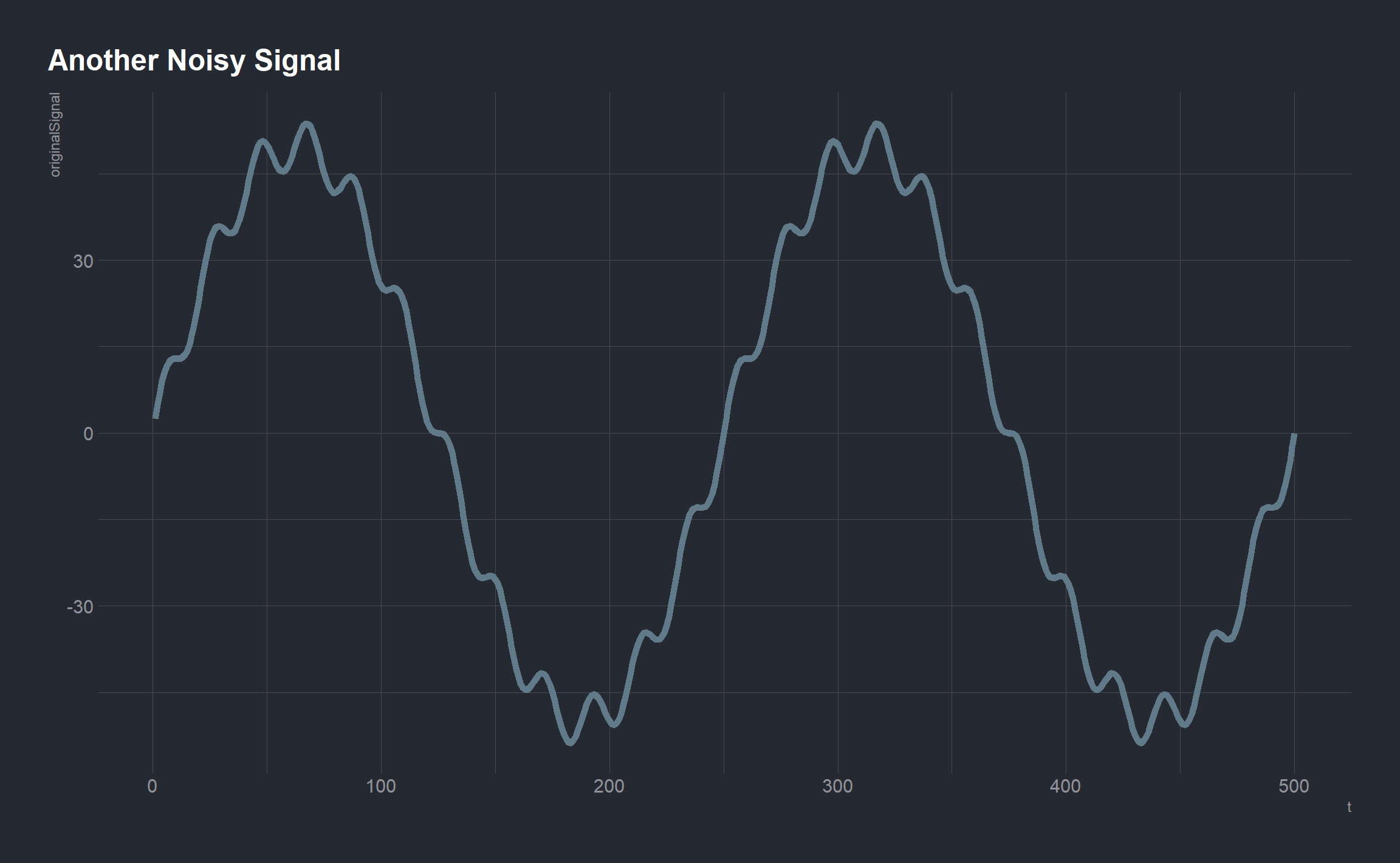

Perhaps we are interested in where the noise is coming from and want to analyze the structure of the noise to figure this out. Thus, unlike the previous example, we want to extract the noise from the signal and not simply eliminate it. To do this we can again use the Butterworth filter.

lowButter <- butter(2, 1/50, type = "low")
low <- signal::filter(lowButter, originalSignal)

highButter <- butter(2, 1/25, type = "high")
high <- signal::filter(highButter, originalSignal)

signals <- data.frame(originalSignal, low, high)

ggplot(signals, aes(t)) + 
  geom_line(aes(y = originalSignal, color = "Original")) + 
  geom_line(aes(y = low, color = "Signal")) + 
  geom_line(aes(y = high, color = "Noise")) + 
  labs(x = "Time", y = "Signal",
       title = "Butterworth Filtering")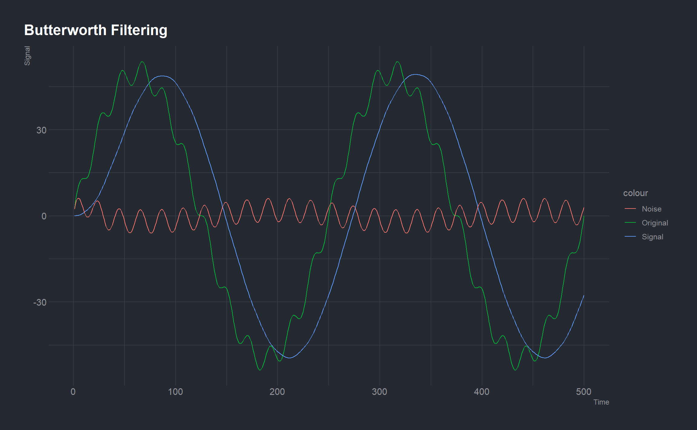

Fourier Transforms and Spectrograms

When working with signals the data can always be depicted in both the time domain and the frequency domain. The most popular way to explore signals in the frequency domain is to use Fourier Transforms. A Fourier Transform is a reversible mathematical algorithm developed by Joseph Fourier in the early 1800s. The transform breaks apart a time series into a sum of finite series of sine & cosine functions.

The Discrete Fourier Transform (DFT) is a specific form of the Fourier Transform applied to a time domain wave. The DFT rebuilds the original time domain continuous wave using frequency and amplitude attributes of the original time series wave form. Fourier Transforms require a window size parameter. Increasing the window size will increase frequency resolution, but this will also make the transform less accurate in terms of time as more signal will be selected for the transform. Thus there is a constant level of uncertainty between the time of the signal and the frequency of the signal. Different windows can be used in a DFT depending on the application. There are numerous windows available that we will explore within the seewave package .

Computing a fourier transform on a whole sound file or a single segment of the sound may not be enough information. Most applications compute the DFT on successive sections along the entire sound signal. A window is “slided” along the signal and a DFT is computed at each of these slides. This process is called a Short-Time Fourier Transform, or STFT.

We can plot the results of an STFT in what is called a spectrogram. The successive DFT are plotted against time with the relative amplitude of each sine function of each DFT represented by some color scale. In other words, the spectrogram has an x-axis of time, a y-axis of frequency, and the amplitude represented by the color scheme used inside the plot. Let’s look at an example:

Speech in the time and frequency domain lab:

In his recent blog post, Eric NTay analyzed a speech signal in the time and frequency domain. The objectives were:

To create a two second recording of one of the 10 digits in Swahili.
To compute a spectrogram of the recorded speech signal.
To obtain a segment 32ms long from a region with speech and another segment of the same duration from a segment without speech, and then plot and analyze them in the time domain.
To compute the Discrete Fourier, Transform of both signals in (c) above.

The Discrete Fourier Transform (DFT) is considered as the frequency domain representation of the original input sequence. The DFT is itself a sequence rather than a function of a continuous variable, and it corresponds to samples, equally spaced by frequency. A continuous time signal x(t) is first sampled to form the discrete time signal x[n] of length N samples. The transformed signal within the frequency domain is of finite extent but discrete and of the same length as the original signal. The DFT then decomposes a time domain signal defined over a finite range into a sum of weighted complex sinusoids as:

\(X(k) =\sum_{n=0}^{N-1} x[n] {e^{-j\frac{2\pi}Nkn}}\)

This operation is useful in many fields but computing it directly from the definition is often too slow to be practical. The fast Fourier transform (FFT) is the algorithm that computes the discrete Fourier Transform of a sequence or its inverse.

Data Analysis in R

Let’s now take a look at how we can analyze the speech signal in the time and frequency domain. The following table lists common feature quantities used in signal processing to characterize and interpret signal properties. They will be quite useful in our analysis:

Quantity	Description
y	Sampled data
N <- length(y)	Number of samples
Fs	Sample frequency (samples per unit time or space)
dt <- 1/Fs	Time or space increment per sample
t <- (seq_len(n) - 1)/Fs	Time or space range for data
dft <- fft(y)	Discrete Fourier transform of data (DFT)
abs(dft)	Amplitude of the DFT
(abs(dft)^2)/N	Power of the DFT
Fs/N	Frequency increment/Frequency resolution
f <- (seq_len(n) - 1)*(Fs/N)	Frequency range

A single channel audio signal of the word moja (Swahili word for digit one) sampled at 8 kHz was recorded using a Raspberry Pi and stored as a .wav file. The recording can also be done using a laptop or mobile phone too.

If you would like to follow along using the audio file Eric used in his analysis, download it from here: moja wav

Loading the audio data and some pre-processing

Let’s begin by loading the speech signal recorded, reading it and then rescaling the amplitude of the waveform to a canonical interval [-1,1].

one = here('content/post/DigitalSignalProcessing/moja.wav') 

moja_wave <- tuneR::readWave(one) %>%
  tuneR::normalize(unit = c("1"), center = FALSE, rescale = FALSE)

The audio signal was recorded for 2 seconds and then reduced to a discrete time signal by sampling at 8 kHz to obtain 16000 samples as below:

\(sampling \, period \, (T_s) =\, \frac{1}{sampling\,frequency \, (F_s)} \, =\, \frac{1}{8000}\)

\(T_s \, = \,0.125\, _{ms} \, (time\,difference\,between\,samples)\)

\(Number\,of\,samples\, = segment\,length(sec) \times sampling\,frequency \,\)

\(Number\,of\,samples\, = \,16000\)

All these summaries of the Wave-object can be obtained as:

summary(moja_wave)

## 
## Wave Object
##  Number of Samples:      16000
##  Duration (seconds):     2
##  Samplingrate (Hertz):   8000
##  Channels (Mono/Stereo): Mono
##  PCM (integer format):   TRUE
##  Bit (8/16/24/32/64):    32
## 
## Summary statistics for channel(s):
## 
##    Min. 1st Qu.  Median    Mean 3rd Qu.    Max. 
## -0.5783 -0.0275  0.0031 -0.0010  0.0297  0.7630

Plotting the audio data

Let’s make a plot of the signal’s amplitude vs the corresponding sample number.

# extracting sampled data, y
y = moja_wave@left

# extracting the sample rate, Fs
Fs = moja_wave@samp.rate

# getting our ggplot on
ggplot(mapping = aes(x = seq_len(length(y)), y = y)) +
  geom_line(color = 'blue') +
  labs(x = "Sample Number", y = "Amplitude", title = "Speech waveform")

Take a moment and listen to the audio:

audio::play.audioSample(y, Fs)

From the Speech waveform plot, one can easily identify the segments that contain speech and those without (very faint speech).

We’ll need these segments for some later analysis, so let’s define sample numbers that contain speech and those without.

# sample index of segments with speech and those without
speech_start <- 5100
silence_start <- 9850

Computing a spectrogram of the signal

A spectrogram is a visual representation of the spectrum of frequencies of a signal as it varies with time. It is usually depicted as a heat map with intensity being shown by varying the color or brightness.

We will compute the spectrogram by dividing the speech signal into segments 32ms long (256 samples at 8kHz) with 50% overlap between neighboring segments and taking the FFT of each segment.

We will then plot the magnitude of this FFT for all the segments as a 2-dimensional image showing how the frequency varies with time. ggspectro {seewave} (an alternative to spectro {seewave}) allows us to draw a spectrogram with the package ggplot2. Note is that a Fourier Transform window is specified and that the Fast Fourier Transform (by setting fftw = TRUE) is used to speed up the process.

# defining the window size (number of samples in a 32ms long segment)
N <- 32e-3*Fs

ggspectro(y, Fs, wl = N, wn = "hamming", ovlp = 50, fftw = TRUE) + 
  geom_tile(aes(fill = amplitude)) +
  scale_fill_gradientn(colors = pal,
                       aesthetics = c("fill")) +
  labs(title = "Audio Spectrogram, Moja Speech Waveform",
       subtitle = "32e-3 Window size")

The spectrogram appears as a heatmap with the various colors representing power in decibels. It is evident that the digit was spoken in the interval between 0.4s and 1s where there are high values of frequency.

Now, let’s divide the speech signal into 64ms segments, take the FFT of each segment, and build another spectrogram.

# defining the window size (number of samples in a 32ms long segment)
N_2 <- 64e-3*Fs

ggspectro(y, Fs, wl = N_2, wn = "hamming", ovlp = 50, fftw = TRUE) +
  geom_tile(aes(fill = amplitude)) +
  scale_fill_gradientn(colors = pal,
                       aesthetics = c("fill")) +
  labs(title = "Audio Spectrogram, Moja Speech Waveform",
       subtitle = "64e-3 Window size")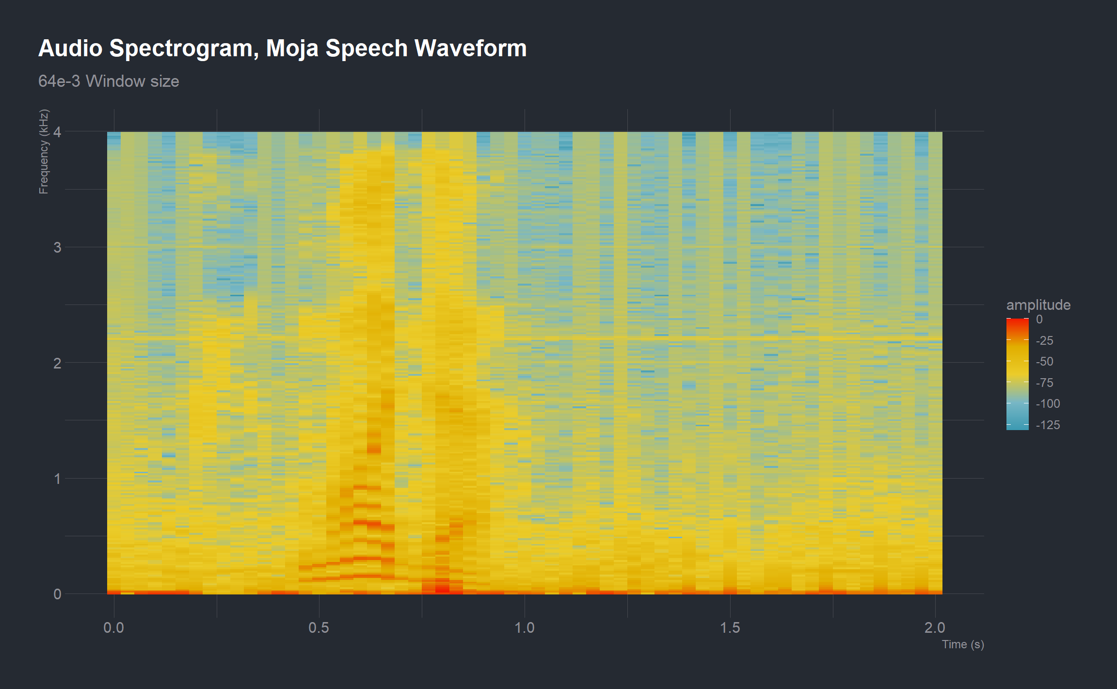

Increasing the segment length to 64ms consequently increases the window length to 512 samples. This effect of this is that the frequency resolution increases. The frequency resolution is obtained by the ratio Fs/N. So, for a given sampling frequency (Fs), the more samples (N) in the signal, the smaller the frequency increment between successive DFT data points. Since more points are being sampled, the spectral resolution increases.

In what frequency range is most of the energy of the signal?

To answer this question, we will have to come up with a magnitude spectrum of the speech waveform which shows the magnitude of the signal at a particular frequency. This means we will have to convert the signal from the time domain to a representation in the frequency domain by computing the Discrete Fourier Transform (using a FFT algorithm).

Due to mathematical convenience, the arrangement of the FFT output has positive and negative frequencies side by side in a slightly non-intuitive order (the frequency increases from 0 until N/2 and then it decreases for negative frequencies). As the positive and negative frequency magnitudes are identical for a real signal it is common just to plot the positive frequencies from 0 to Fs/2 (in our case 0 to 4000 Hz).

# Discrete Fourier transform of data (DFT)
dft_speech <- fftw::FFT(y)

# amplitude of DFT
dft_amp <- abs(dft_speech) # DFT is a sequence of complex sinusoids 

# number of samples
n <- length(y)

# frequency range
f <- (seq_len(n) - 1)*Fs/n

ggplot(mapping = aes(x = f[1:Fs], y = dft_amp[1:Fs])) +
  geom_line(color = 'blue') +
  scale_x_log10() +
  labs(x = "Frequency (Hz)", y = "Magnitude",
title = "Frequency domain representation",
subtitle = "Entire speech sequence")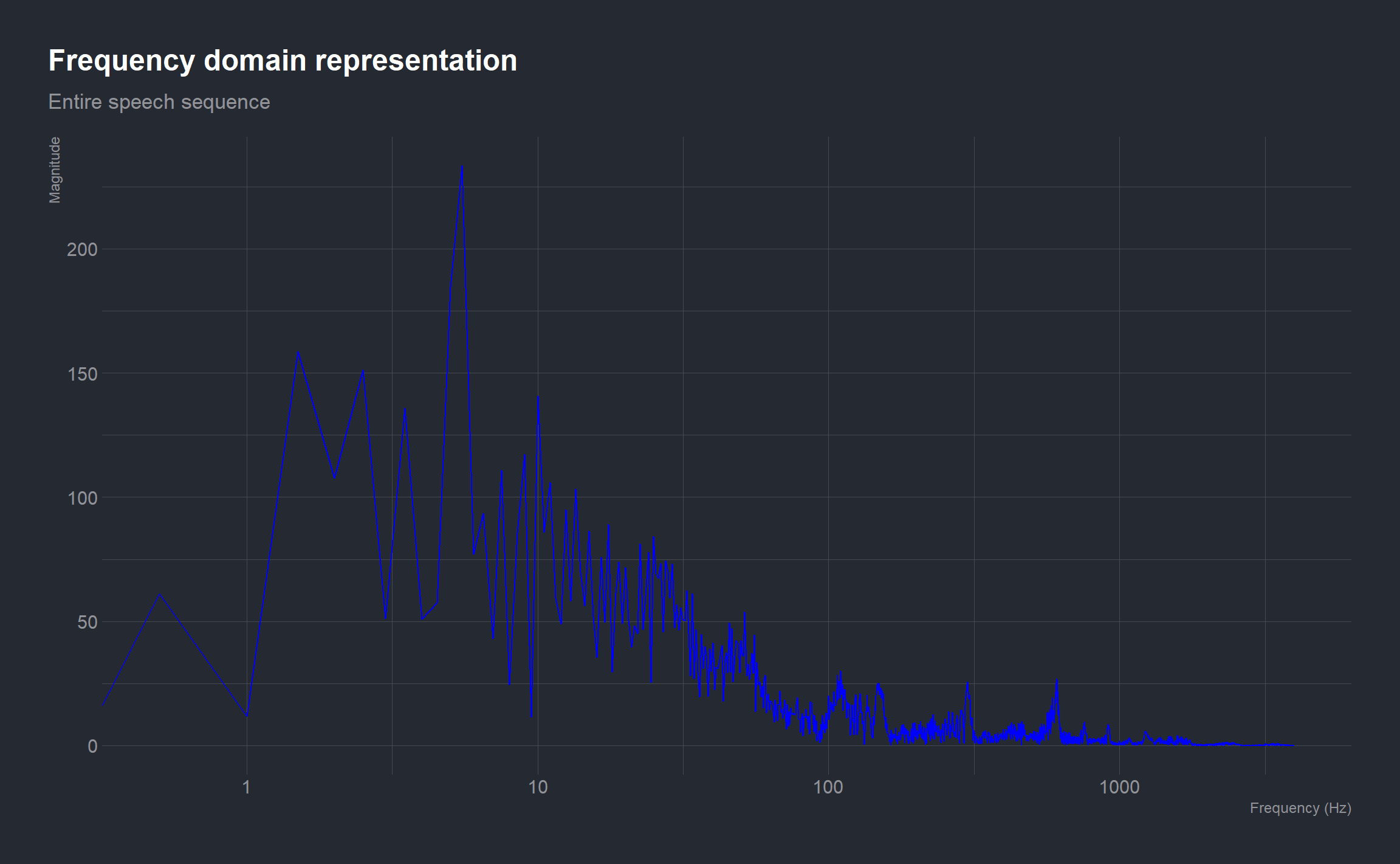

From the magnitude spectrum of the Discrete Fourier Transform, we can observe that most of the energy is concentrated in the frequency range 1 to 10 Hz.

Time domain, Frequency domain and Energy comparison of a segment containing speech and one without

The time domain representation of a speech signal shows how the sound changes in intensity over time

Earlier on in this analysis, we defined some sample numbers in regions containing speech and those without. First, we’ll obtain a segment 32ms long from a region with speech and another segment of the same duration from a segment without speech and plot these time domain signals side by side with time in seconds as the x-axis. A 32ms long segment corresponds to 256 samples:

\(Number\,of\,samples\, = \,segment\,length(sec) \times sampling\,frequency \,\)

\(= 0.032 \times 8000 = 256\)

# sample length
sample_len = 32e-3*Fs

# obtaining a 32ms long segment/256 samples without speech
moja_sl <- y[silence_start:(silence_start + sample_len - 1)]

# obtaining a 32ms long segment/256 samples with speech
moja_sp <- y[speech_start:(speech_start + sample_len - 1)]

# corresponding time-length of the sample (32ms long)
t <- (seq_len(sample_len) - 1) * 1/Fs

# plotting the waveform of the silent segment
wvfm_sl <- ggplot(mapping = aes(x = t, y = moja_sl)) +
  geom_line(color = 'blue', lwd = 1.1) +
  labs(x = "Time (s)", y = "Amplitude",
       title = "Silent Segment",
       subtitle = "Time Domain") +
  scale_y_continuous(limits = c(-0.25, 0.25))

# plotting the waveform of the segment with speech
wvfm_sp <- ggplot(mapping = aes(x = t, y = moja_sp)) +
  geom_line(color = 'blue', lwd = 1.1) +
  labs(x = "Time (s)", y = "Amplitude",
       title = "Speech Segment",
       subtitle = "Time Domain") +
  scale_y_continuous(limits = c(-0.25, 0.25))

cowplot::plot_grid(wvfm_sl, wvfm_sp)

From the above plots above, the time domain plot of the segment containing speech has higher intensity (amplitude ranging from -0.27 to 0.24) than that without speech/faint speech due to noise (amplitude ranging from -0.02 to 0.06).

The time domain plot of the segment containing speech is also more erratic due to more fluctuations in amplitude of sound.

One common metric that can be easily computed from the sample values is a signal's energy.

The energy of a discrete time signal is defined as the sum of the square of the sampled signal values: \(E(y) =\sum_{n=-\infty}^{\infty} y^2\)

# Energy of silent segment
E_sl <- sum(moja_sl^2)
E_sl

## [1] 0.1733

# Energy of segment with speech
E_sp <- sum(moja_sp^2)
E_sp

## [1] 3.441

The silent segment has an energy of 0.1733 whereas the segment containing speech has an energy of 3.4409. Due to higher intensities of sound in the region containing speech, the sample values in this region have higher amplitude values which in turn account for the higher energy. The energy in the silent segment could be attributed to noise and can be filtered out using an appropriate filter.

The time domain analysis can also be done in the frequency domain by computing the Discrete Fourier Transform (using a FFT algorithm) of the two segments.

# DFT of silent segment
dft_sl <- fftw::FFT(moja_sl)

# DFT of speech segment
dft_sp <- fftw::FFT(moja_sp)

# frequency range
fs <- (seq_len(sample_len) - 1)*Fs/sample_len

# plotting the waveform of the silent segment in freq domain
freqd_sl <- ggplot(mapping = aes(x = fs[1:(sample_len)/2],
  y = abs(dft_sl[1:(sample_len)/2]))) +
  geom_line(color = 'blue', lwd = 1.1) +
  labs(x = "Frequency (Hz)", y = "Amplitude",
       title = "Silent Segment",
       subtitle = "Frequency Domain") +
  scale_x_log10()

# plotting the waveform of the speech segment in freq domain
freqd_sp <- ggplot(mapping = aes(x = fs[1:(sample_len)/2], 
  y = abs(dft_sp[1:(sample_len)/2]))) +
  geom_line(color = 'blue', lwd = 1.1) +
  labs(x = "Frequency (Hz)", y = "Amplitude",
       title = "Speech segment",
       subtitle = "Frequency Domain") +
  scale_x_log10()

cowplot::plot_grid(freqd_sl, freqd_sp)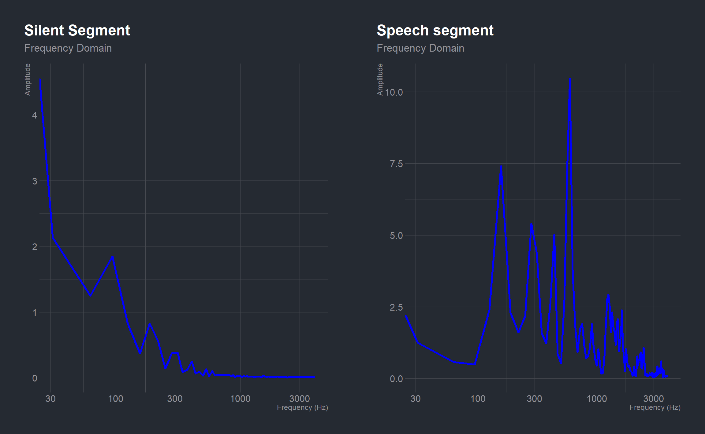

When the two segments are converted from the time domain to a representation in the frequency domain the same inferences made earlier still hold. The segment containing speech has higher magnitude than that without speech at various frequencies.

Signal power as a function of frequency is another common metric used in signal processing. Power is the squared magnitude of a signal’s Fourier transform, normalized by the number of frequency samples:

\(P_{dft}\, =\, [\mid {(dft)}\mid^2]/N\)

A power spectrum of the segment containing speech:

# power of the dft
power <-  ((abs(dft_sp))^2)/sample_len

# frequency range
fp <- (seq_len(sample_len) - 1)*Fs/sample_len

ggplot(mapping = aes(x = fp[1:(sample_len)/2],
  y = power[1:(sample_len)/2])) +
  geom_line(color = 'blue', lwd = 1.1) +
  labs(x = "Frequency (Hz)", y = "Power",
       title = "Power Spectrum of speech segment") +
  scale_x_log10()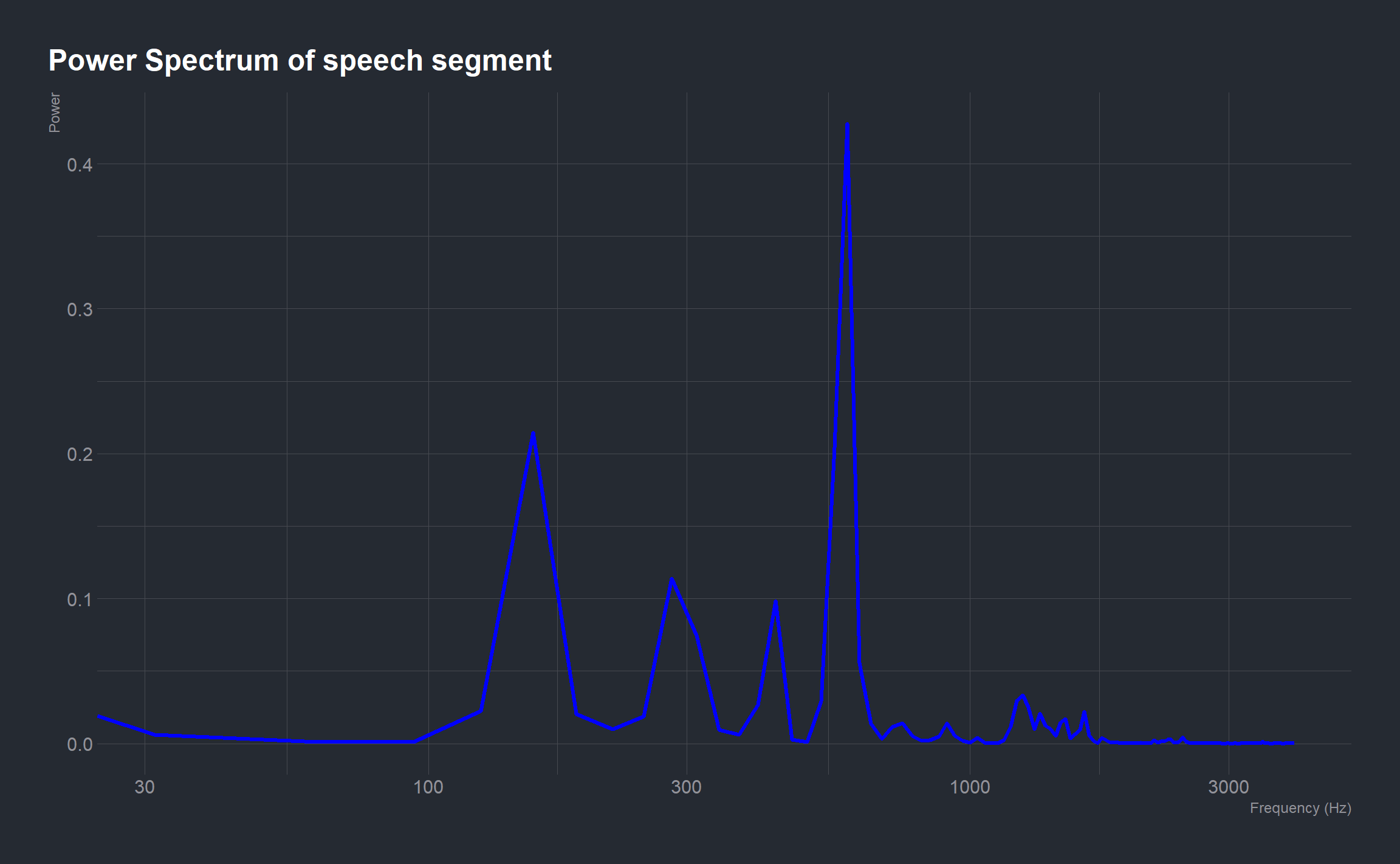

The plot indicates that the speech segment consists of a fundamental frequency around 156.25 Hz and a sequence of harmonics, where the third harmonic is emphasized.

EnsembleML is an R package for performing feature creation in time series and frequency series, building multiple regression and classification models and combining those models to be an ensemble. Features can be created both in time domain and frequency domain.

# Features of the moja_wave 
featureCreationF(y)

##    F_mean  F_sd F_median F_trimmed  F_mad    F_min F_max F_range F_skew F_kurtosis
## X1  2.669 8.454   0.5853     1.129 0.7326 0.001252 233.5   233.5  10.81      176.7
##       F_se F_iqr F_nZero F_nUnique F_lowerBound F_upperBound   F_X1.   F_X5. F_X25.
## X1 0.09451 1.931       0      8000       -2.699        5.026 0.01723 0.03317 0.1982
##    F_X50. F_X75. F_X95. F_X99.
## X1 0.5853  2.129  10.54  36.04

The standard features include mean, sd, median, trimmed, mad, min, max, range, skew, kurtosis, se, iqr, nZero, nUnique, lowerBound, upperBound, and quantiles. Others could be defined.

Other Resources:

The fftw package provides a wrapper around the fast, award winning FFTW library of C subroutines developed at MIT. The dlm package for fitting Maximum Likelihood and Bayesian dynamic linear models includes dlmFilter(), a flexible function based on singular value decompositions for Kalman filtering. The vignette for the dlm package provides a brief introduction to the underlying theory which is further developed in the Springer book Dynamic Linear Models with R by Campagnoli, Petrone and Petris.

R and Signal Processing
R Programming for Data Sciences
Eric NTay’s blog post at A gentle introduction: R in Digital Signal Processing
Nagdev Amruthnath’s talk at Big Data Ignite 2020 on his {EnsembleML} package
Bioacoustics in R with warbleR